I’m working on a remix of a short 5 channel piece constructed from the sounds of gas-filled ping pong balls. (From this excellent Daniel Blinkhorn album.)

The original (Gossima Collective 1) has such shape in its 98 seconds. There’s so much going on without ever collapsing into mush. It’s a really wonderful piece of microsound.

My general approach to the remix so far is to extract information from the original to drive a little ensemble of embodied instruments, and maybe play along on trombone or trumpet if I’m feeling confident enough.

I haven’t finished wiring up the solenoid/motor driver module for my instrument yet, so I might end up using a bank of relays I bought on the internet that can be controlled over wifi via an embedded esp32 for this while I work on that.

Today I started trying to mine the source for signals. Pippi wraps some of the wonderful librosa library’s music information retrieval functionality in the mir module. Running each of the 5 source tracks through it to extract a wavetable following spectral bandwidth, flatness, rolloff, centroid, and contrast and seeing what seems interesting and useful was basically the name of the game today.

I have a hard time hearing the difference between the individual channels of the surround mix, but many of these MIR routines revealed some really rich differences while still being correlated. For example: I used the spectral bandwidth curves for modulating durations, and spectral contrast as an FM modulator in places. These both had really cool correlations between the tracks without being totally aligned – sometimes differing starkly.

Here’s an example of the spectral bandwidth curve from the first two channels of the source:

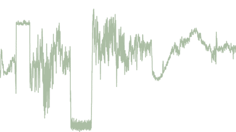
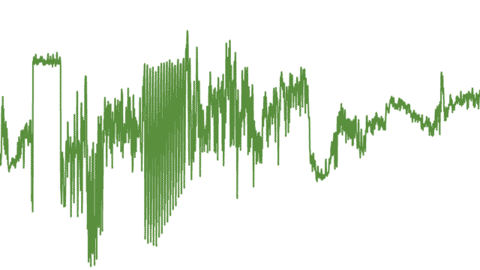
There is a general kind of alignment, but also lots of local variation. Sometimes there are total shifts like that section at the end of the first half which pins to a tight oscillation in the first channel and varies widely in the second.

This is all very preliminary, and I haven’t even started trying to work in the solenoids and motors yet. Some shapes are starting to emerge though, maybe.

As seems typical the tests I’ve done today are way too dense and uniform. I might try drawing some subjective curves by hand based on listening to the original too, to try to capture the shape of it.

I also want to think about harmony – the original teases it wonderfully and I’d like to expand on that, especially if I’m going to work some trombone into it eventually.

For now the script I cobbled together today uses randomness to reduce the density a bit, and I just slapped some harmony onto it to see how it would sound.

One of the best lessons I took away from studying with JM was: don’t be afraid to break your own rules. So, keeping in mind that I want to try to derive the shapes and particulars from the signals embedded in the original, I plan to also try to explore the spirit of it in the end and break some rules if needed. :)

Here’s the pippi script from today’s experiments. This writes a 5 channel file to disk. To test I was using an astrid script that remixes it to 4 channels (though I’ll eventually go to 5 when I bring another amp to my office) – I was surprised to find it seems difficult to get sox or aplay or oceanaudio or any linux program I tried to just emit N channels if there isn’t a corresponding N channel soundcard available. I was sending audio through the built-in headphone jack and another stereo dongle for this.

from pippi import dsp, oscs, mir, fx, shapes, tune

srcs = dsp.readall('g1*.wav')

freqs = tune.degrees([1,2,3,4,5,6,7,8,9], octave=3)

layers = []
for i, src in enumerate(srcs):
    env = src.toenv().autoscale(0, 1)

    bw = mir.bandwidth(src)
    bw = bw.toenv().autoscale(0.5, 3)

    flat = mir.flatness(src)

    cent = mir.centroid(src)

    roll = mir.rolloff(src)

    cont = mir.contrast(src).autoscale(0.5, 2)

    pitch = mir.pitch(src)
    pitch = pitch.autoscale(0.01, 1)

    onsets = mir.onsets(src)
    layer = dsp.buffer(length=src.dur, channels=1)
    for o in onsets:
        durmul = bw.interp(o/src.dur)
        freqmul = pitch.interp(o/src.dur)
        maskmul = cont.interp(o/src.dur)

        seg = src.cut(o, dsp.MS*100).remix(1)
        freq = mir.centroid(seg).remix(1).avg * freqmul
        mask = mir.contrast(seg).remix(1) * maskmul
        dur = mir.flatness(seg).remix(1).mag
        bit = oscs.SineOsc(freq=freq*mask).play(dur*durmul).env('hannout') * seg.mag
        if dsp.rand() > 0.5:
            layer.dub(bit, o*durmul)

        if dsp.rand() > 0.5:
            layer.dub(seg.speed(freqmul*10).env('hannout')*3, o*durmul)

        if dsp.rand() > 0.8:
            if dsp.rand() > 0.5:
                ws = dsp.ws(seg)
            else:
                ws = dsp.ws(seg, limit=dsp.randint(4,40))

            for _ in range(dsp.randint(2,6)):
                tone = oscs.Pulsar2d(ws, freq=dsp.choice(freqs)).play(dur*durmul*dsp.rand(3,10)).env('hannout') * seg.mag * 2
                layer.dub(tone, o*durmul)

    layer.write(f'o{i}.wav')
    #layer = layer.remix(2).pan(i/len(srcs))
    layers += [ layer ]

out = dsp.stack(layers)
out = fx.norm(out, 0.8)
out = out.trim()
out.write('mixed.wav')

Here’s the little astrid playback script for good measure. I think ultimately I’ll pre-render most of the shapes and then do the synthesis via astrid’s just-in-realtime scheme to make syncronizing with solenoids / motors easier.

from pippi import dsp
import astrid

def play(ctx):
    mix = dsp.read('mixed.wav')
    return mix.remix(4)

if __name__ == '__main__':
    astrid.run_forever(__file__, output_channels=4)

Log July 2026